
Beer-Lambert Law and Cuvette Selection: A Practical Guide
This post is also available in:
Beer-Lambert Law
Beer-Lambert Law & Cuvette Selection: A Practical Guide
The single equation behind every quantitative UV-Vis measurement — and the cuvette decisions that determine whether your readings stay within its valid range.
A = ε · c · L
Absorbance = (molar absorptivity) × (concentration) × (path length)
The Beer-Lambert law is the linear relationship between absorbance, analyte concentration, and optical path length expressed as A = ε · c · L, where ε is molar absorptivity (L·mol⁻¹·cm⁻¹), c is concentration (mol·L⁻¹), and L is path length (cm). It accurately predicts UV-Vis absorbance for dilute, non-scattering solutions in the 0.1–1.0 absorbance range; outside this window, deviations from linearity become significant and require correction.
Definition
The Beer-Lambert law (also called the Beer-Bouguer-Lambert law or the Beer-Lambert-Bouguer law) states that the absorbance of light through a sample is the product of three quantities: the molar absorptivity (ε) of the analyte, the molar concentration (c) of the absorbing species, and the optical path length (L) through the sample. Mathematically: A = ε · c · L. The law holds reliably for dilute solutions of non-interacting absorbers in the absorbance range 0.1–1.0 AU; outside this range, deviations from linearity become significant and must be corrected.
Foundation
The equation, units, and what each variable means
A = ε · c · L
- A
- = absorbance (unitless, also written OD or “optical density”) ·
- ε
- = molar absorptivity, units L·mol⁻¹·cm⁻¹ (also called extinction coefficient) ·
- c
- = concentration of absorbing species, mol·L⁻¹ ·
- L
- = path length, cm
The law links the three controllable quantities in a UV-Vis measurement. Two are properties of the sample (ε is intrinsic to the molecule + solvent + wavelength; c is what you’re trying to measure or control). The third — path length L — is set by your cuvette choice. Selecting the right cuvette is therefore a Beer-Lambert decision.
An equivalent form expressed via transmittance:
A = −log₁₀(I / I₀) = −log₁₀(T)
Where I₀ is the intensity entering the sample, I is the intensity transmitted, and T is fractional transmittance (0–1). An absorbance of 1.0 = 10 % transmission, A = 2.0 = 1 %, A = 3.0 = 0.1 %.
Valid Range
Where the Beer-Lambert law actually holds
The textbook equation assumes a list of conditions that real samples often violate. Honest practice keeps measurements inside the valid window:
- Monochromatic light — instruments use a finite spectral bandwidth. If the bandwidth is wider than the absorption peak, apparent ε flattens and linearity bends down.
- Non-scattering, non-fluorescent sample — turbid suspensions, micelles, and strongly fluorescent dyes break the simple absorbance accounting.
- Dilute, non-interacting absorbers — at high concentrations (typically > 10 mM for small organic molecules), molecules begin to associate, dimerize, or change refractive index of the solvent — all of which alter ε.
- Stable detector linearity — most UV-Vis detectors are linear from 0.005 to 2.0 AU. Above 2.0 AU, stray light begins to dominate the readout.
- Non-zero path length — the law assumes a defined L. In flow cells with poor optical alignment, the effective path length may not equal the nominal value.
| Absorbance Range | Behavior | Action |
|---|---|---|
| A < 0.05 | Detector noise dominates | Use longer path length to boost signal |
| 0.1 ≤ A ≤ 1.0 | Linear, optimal range | No change needed |
| 1.0 < A ≤ 2.0 | Slight non-linearity, stray light starts | Acceptable for most work; verify with standards |
| A > 2.0 | Severe non-linearity, stray light dominates | Dilute sample OR use shorter path length |
| A > 3.0 | Effectively unmeasurable on standard UV-Vis | Always dilute or switch instrument |
The Cuvette Decision
Why path length is the cuvette designer’s lever on Beer-Lambert
If you can’t change ε (the molecule), and you don’t always want to change c (your sample as-is), the only Beer-Lambert variable you can manipulate at the bench is L — and L is exactly the cuvette path length.
The same sample measured in different cuvettes gives different absorbance values. A protein at 1 mg/mL with ε = 1.0 mL·mg⁻¹·cm⁻¹ at 280 nm gives:
| Cuvette Path Length | Measured Absorbance | Interpretation |
|---|---|---|
| 0.1 mm (sub-mm cuvette) | 0.01 AU | Below noise floor — bad |
| 1 mm (UPLC flow cell) | 0.10 AU | Just above noise — OK if quick measurement |
| 10 mm (standard cuvette) | 1.00 AU | Center of valid range — ideal ✅ |
| 100 mm (long-path cell) | 10.0 AU | Saturated — unreadable, dilute sample |
Same sample, four different answers — three of which are wrong. The cuvette choice is the measurement quality decision. For a working table of which cuvette path length to use for which analyte concentration range, see our path-length-by-analyte selection matrix.
Worked Example — Diluting vs Switching Cuvettes
You measure a UV-Vis sample at A = 2.4 AU in a 10 mm cell. Two paths to a valid reading:
Option A — Dilute 5×: A drops to 0.48 AU. Easy if you have sample volume to spare; introduces a ~2 % dilution error per step.
Option B — Switch to 1 mm cell: A drops to 0.24 AU. No dilution, no propagated error. Same exact sample.
For trace analyses, scarce samples, or kinetics where you can’t afford to disturb the sample, Option B is dramatically better. This is why MachinedQuartz stocks sub-millimeter cuvettes down to 0.01 mm path length.
Path length range — same A = ε·c·L, four cuvettes
Pick the cuvette that places A in the linear range
C052CF2
Quartz 5mm Standard Cuvette
C105CS
Quartz 10mm Standard Cuvette
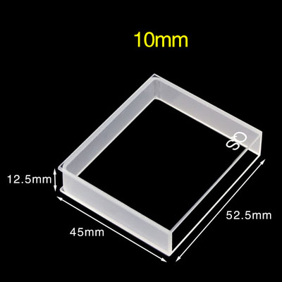
C502CL
Quartz 10mm Path / 50mm Body Large
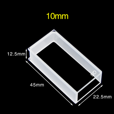
C202CE9
Quartz 20mm Standard Cuvette
Same sample, same ε, same c — only L differs. Move from saturated to noisy by changing the cell, not the chemistry.
When the Law Fails
Real-world deviations from linearity
Stray light at high absorbance
Stray light is any photon that reaches the detector without passing through the sample as intended — scattered off lens edges, leaked through the beam stop, or reflecting off cuvette walls. In a perfectly designed instrument stray light is < 0.01 %. In a typical bench UV-Vis it’s 0.05–0.5 %.
The effect: at A = 3.0 (transmittance 0.1 %), even 0.05 % stray light contributes half the apparent transmitted signal — your reading is no longer a function of true sample absorbance. The cuvette can contribute too: a poorly polished or scratched cell adds wall scatter that mimics stray light.
Mitigation: Use Sintered 83 or Molded 83 grade cuvettes (T > 83 %, full polish, low stray light). Verify with a known-OD standard at 1.0 and 2.5 AU; if the 2.5 AU reading is < 2.4 AU, your stray light is too high — replace the cuvette or dilute the sample.
Polychromatic radiation and bandwidth effects
If your spectrophotometer has a 5 nm slit width and you’re measuring an absorption peak that’s only 3 nm wide (typical for sharp electronic transitions in lanthanides or transition-metal complexes), the apparent absorbance is averaged over wavelengths where ε differs. The peak appears flatter, and apparent ε drops at high concentrations.
Fix: Narrow the spectral bandwidth to ≤ 0.1× the natural FWHM of your absorption peak. Most modern UV-Vis instruments default to 1–2 nm — adequate for most molecular analytes.
Solute-solute interactions
Above ~10 mM for many small organic dyes, molecules dimerize or form aggregates. The dimer/aggregate has a different ε than the monomer. Apparent A still rises with concentration but no longer linearly — the curve flattens or kinks.
Fix: Stay dilute. If you must measure concentrated samples, use shorter path length (sub-mm cuvettes) so the optical absorbance drops back into the linear regime even though concentration is high.
Refractive index changes
Concentrated solutions have higher refractive index than the solvent blank. This subtly changes the beam geometry and the effective path length within the cell. For most aqueous samples up to 1 M concentration the effect is < 1 %; for concentrated organic solutions or salt brines it can reach 5 %.
Fluorescence emission overlap
If your analyte fluoresces at a wavelength near the absorption measurement, some emitted photons reach the detector and reduce apparent absorbance. Common with fluorescein, rhodamine, and many drug compounds.
Fix: Use a detector with a narrow acceptance angle, or measure at a wavelength outside the emission band. For dedicated fluorescence quantification, use a 4-sided fluorescence cuvette — see our fluorescence cuvette guide.
OD Measurement Best Practice
How to make a defensible OD measurement
“OD” (optical density) is functionally synonymous with absorbance (A) in UV-Vis spectroscopy: OD = −log₁₀(T). A clean OD measurement requires three discipline points:
- Always blank with the same cuvette and same solvent. Use a matched-pair cuvette set if possible — two cuvettes ground from the same blank to ±0.005 AU intrinsic difference. If only one cell is available, blank in that exact cell, then empty and refill with sample without removing it from the holder. See UV-Vis troubleshooting for cell-to-cell offset corrections.
- Measure at λ_max for the highest sensitivity. ε is by definition largest at the absorption peak. Measuring at the shoulder gives smaller signal and more bandwidth-related error.
- Hit the center of the linear range. Aim for 0.3 ≤ A ≤ 1.0. If your sample reads outside this range, either dilute (or concentrate) the sample, or switch path length. Don’t accept a 2.5 AU reading because “the math still works” — the math doesn’t work; stray light contaminates the reading.
Quantification vs detection
For quantification, run a 5-point standard curve in the same cuvette across A = 0.1 → 1.0 and verify R² > 0.999. For detection / qualitative work, a single point at the expected concentration is sufficient. Always report which mode you’re in.
Need a custom path length to put your sample in the linear range?
MachinedQuartz fabricates cuvettes from 0.01 mm to 100 mm path length, custom geometries shipped in 4–6 weeks.
Request Custom Quote Path-by-Analyte ToolFAQ
Frequently asked questions
What is the Beer-Lambert law in one sentence?
The Beer-Lambert law states that the absorbance of a sample equals the product of the analyte’s molar absorptivity, its concentration, and the optical path length through the sample (A = ε · c · L), holding accurately for dilute, non-scattering solutions in the 0.1–1.0 absorbance range.
Is the Beer-Lambert law and the Beer-Bouguer-Lambert law the same?
Yes — these are different historical naming conventions for the same equation. Pierre Bouguer described the path-length dependence in 1729; Johann Lambert refined it in 1760; August Beer added the concentration relationship in 1852. Modern usage treats all three names as synonyms; “Beer-Lambert law” is the most common short form.
What’s the difference between absorbance and OD?
In UV-Vis spectroscopy, absorbance (A) and optical density (OD) are interchangeable — both equal −log₁₀ of the fractional transmittance. “OD” is more common in biology and biochemistry; “absorbance” is the formal IUPAC term. Both are unitless.
At what absorbance does the Beer-Lambert law break down?
The law remains accurate within ±2 % up to about A = 1.0 in most modern instruments. From A = 1.0 to 2.0, deviations grow to 5–10 % primarily from stray light. Above A = 2.0, deviations become severe and unreliable. Always work at A < 1.5 for quantitative work; ideally aim for A = 0.3–1.0.
How does cuvette path length affect Beer-Lambert measurements?
Path length (L) is the only variable in A = ε · c · L that the user can change independently of the sample. Doubling path length doubles absorbance at fixed concentration. To get a too-high reading into the linear range, use a shorter cuvette (e.g. 1 mm instead of 10 mm). To boost a weak signal, use a longer cuvette (e.g. 50 or 100 mm) — though this requires more sample volume.
What is molar absorptivity ε?
Molar absorptivity (also called the extinction coefficient) is an intrinsic property of a compound at a specific wavelength and solvent. Units: L·mol⁻¹·cm⁻¹. It quantifies how strongly the compound absorbs light. Common values range from ~10 (weak transitions in transition metal complexes) to > 100,000 (intense π-π* transitions in conjugated dyes). Look it up from literature for your specific molecule and wavelength.
Can I use the Beer-Lambert law for fluorescence?
Not directly. Fluorescence emission intensity follows a similar but distinct relationship (F ∝ I₀ · ε · c · L · Φ for low absorbance) where Φ is the quantum yield. Beer-Lambert governs the absorption step; the fluorescence step adds a separate efficiency term. For fluorescence quantification, use a 4-sided polished cuvette and measure at the emission maximum.
Why does my absorbance reading drift over time?
Common causes: (1) bubbles forming in the cuvette as the sample warms — degas the sample; (2) photodegradation of the analyte under the measurement beam — minimize beam exposure or use a kinetics mode; (3) the lamp warming up — let the instrument run for 30 min before precise measurements; (4) cuvette contamination — re-blank with a fresh aliquot of solvent. See our UV-Vis troubleshooting guide for the full diagnostic flow.
Read related content
Pair this guide with our path-length-by-analyte matrix and cuvette selection guide for full coverage.
Cuvette Selection Guide Path by Analyte

Recent Comments